Self-Supervised Micrograph Quality Assessment (prismPYP)¶

prismPYP is a label-free pipeline for classifying cryo-EM micrographs using both real-space and Fourier-space features, as described in He and Bartesaghi (2026).

The prismPYP workflow in nextPYP operates on real domain and Fourier domain images as two independent branches that can be run in parallel. In each branch, we perform dataset-specific feature learning and use the trained model to produce visualization results in both 2D and 3D.

Model training and inference (in 2D and 3D) are performed in the Pre-processing block
After a selection of high-quality images has been made, “consensus filtering” is performed as the first step in the Particle refinement block

Pre-requisites¶

Visualization¶

To analyze the results of prismPYP interactively, you need to install and run Phoenix-Arize on your local machine.

For a local installation on macOS, follow these steps:

Download and install Miniconda following these instructions
Activate the Miniconda installation, create a new conda environment and install Phoenix:

source ${INSTALLATION_PATH}/miniconda3/bin/activate
conda create -n phoenix -c conda-forge python=3.8 pip
conda activate phoenix
mkdir prismpyp_phoenix
cd prismpyp_phoenix
wget https://raw.githubusercontent.com/nextpyp/prismpyp/refs/heads/main/requirements-phoenix.txt -O requirements-phoenix.txt
python -m pip install -r requirements-phoenix.txt

Data pre-processing¶

prismPYP operates on frame-aligned and CTF-corrected micrographs. Consequently, it is run as the last step of the Pre-processing block. For examples of how to pre-process single-particle data in nextPYP, see the single-particle tutorial.

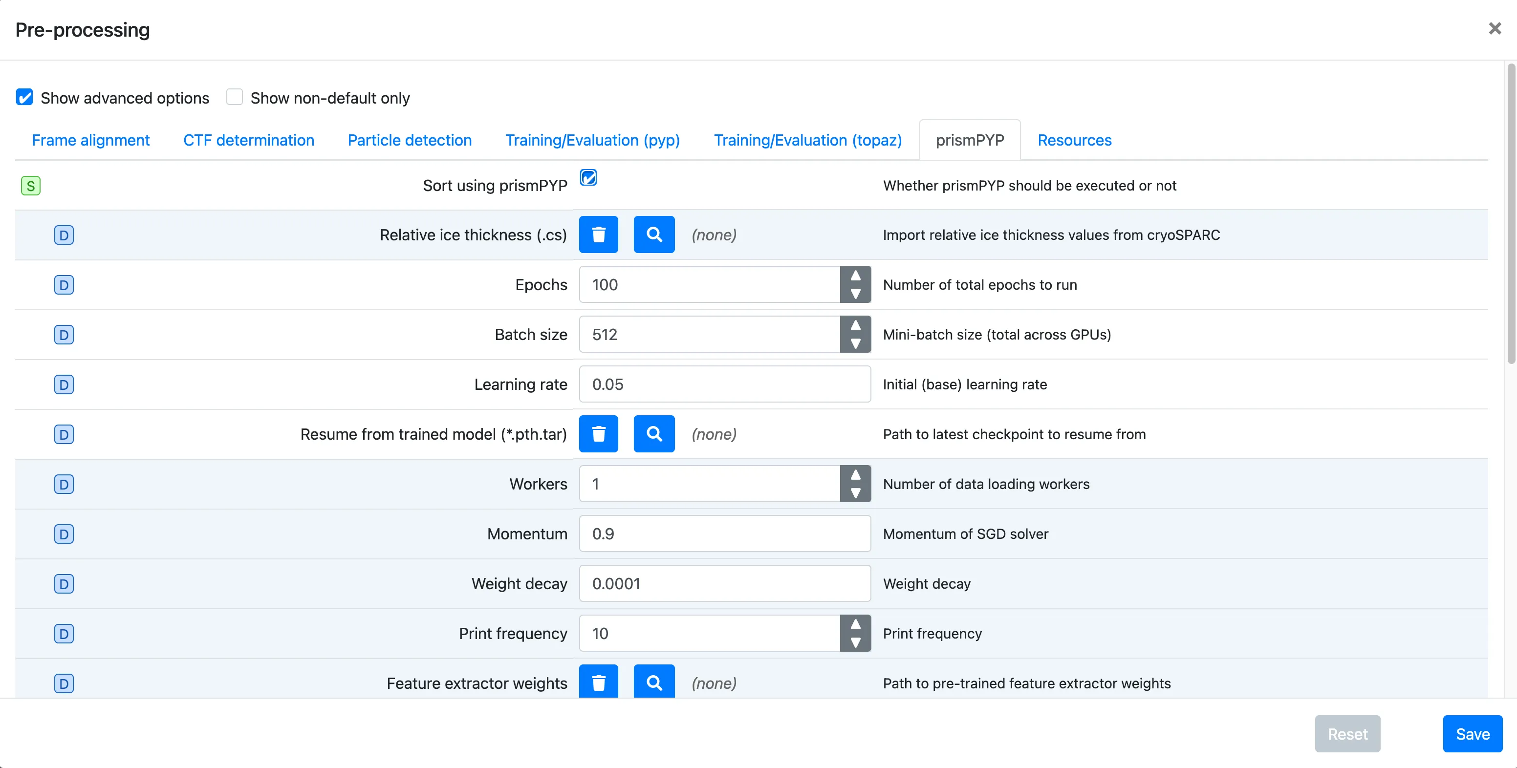
Click on the prismPYP tab
Click on Sort using prismPYP to enable training and inference.
If you have pre-processed the data in cryoSPARC and have the corresponding .cs results, you can import them using the Relative ice thickness (.cs) field by clicking on the icon and navigating to the directory where the file is available. For more information on processing your data in cryoSPARC for prismPYP, see these instructions.
Set the training parameters as needed. You can find more information about parameters used for training, 2D evaluation, and 3D evaluation by clicking on the hyperlinks.
To provide a path to the pre-trained ResNet-50 backbone weights, click on the icon next to Resume from trained model (*.pth.tar) and navigate to the directory where the weights were downloaded (e.g., pretrained_weights/).
Click Save, Run, and Start Run for 1 block

Note

In order for training to run successfully, you must ensure that your Batch size is less than the number of images present in your dataset.
In order for K-Means clustering to run successfully, you must ensure that your KMeans clusters parameter is less than the number of images in your dataset.
In order for UMAP dimensionality reduction to run successfully, you must ensure that your UMAP neighbors parameter is less than the number of images in your dataset.

Visualizing the learned embedding space (in nextPYP)¶

Once the model has finished generating embeddings for the images in your dataset, you can navigate inside the Pre-processing block and click on the prismPYP tab.

We can view the results for the Real space and Fourier space models by clicking on the tabs at the top of the page:

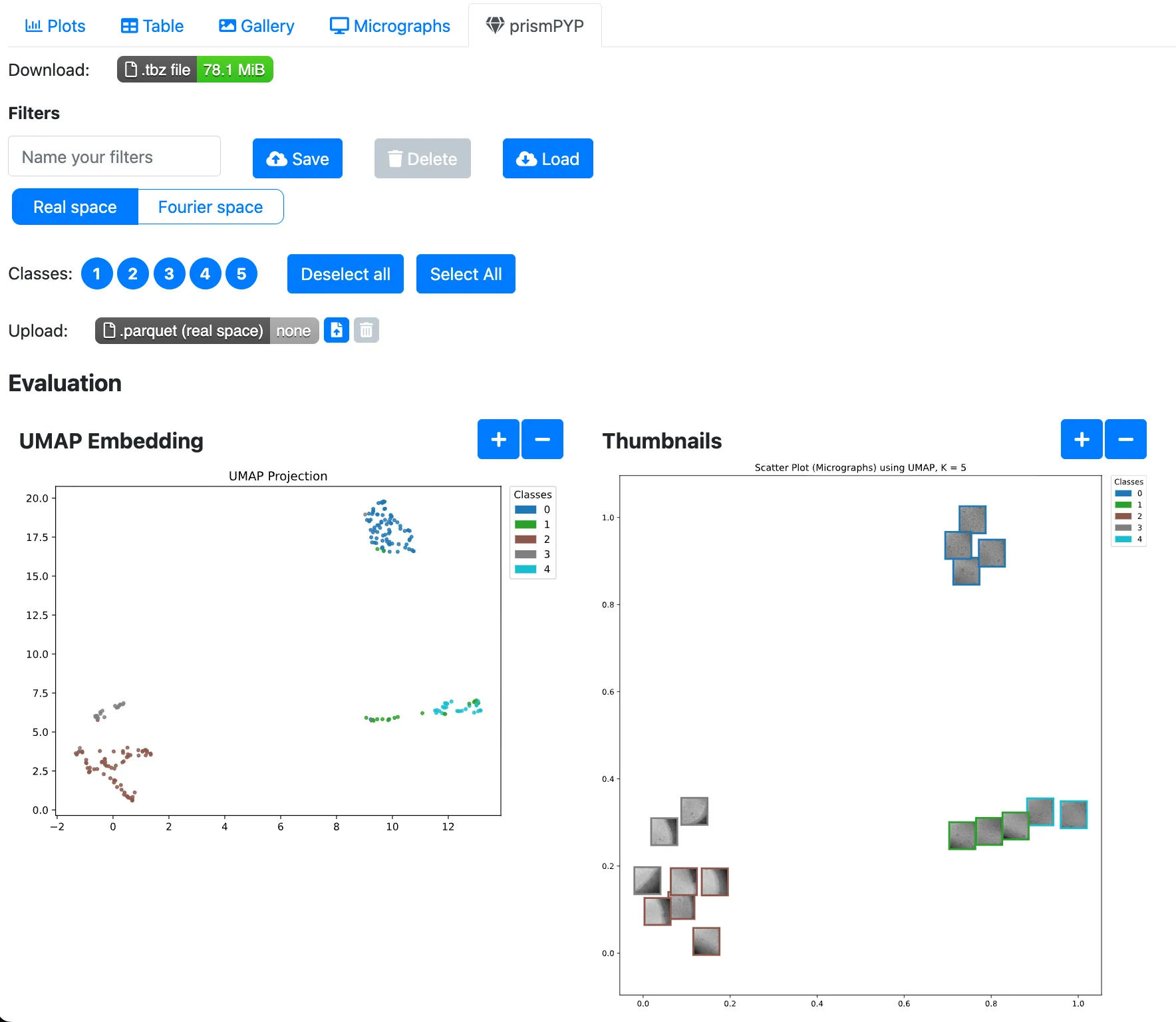
Running inference in 2D will generate two static 2D UMAP plots. The plot on the left represents each image as a colored dot that corresponds to its class as determined by K-Means. The plot on the right shows a thumbnail preview of each image.
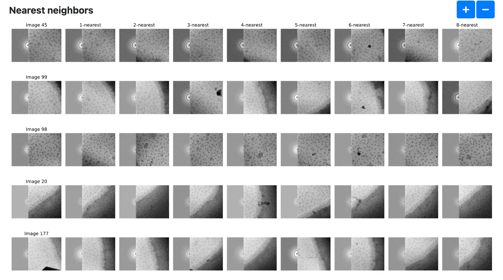
In addition, we can also show an image and its k nearest neighbors. The Number of images to show nearest neighbors and Number of nearest neighbors options in the prismPYP settings tab controls how many images are shown.

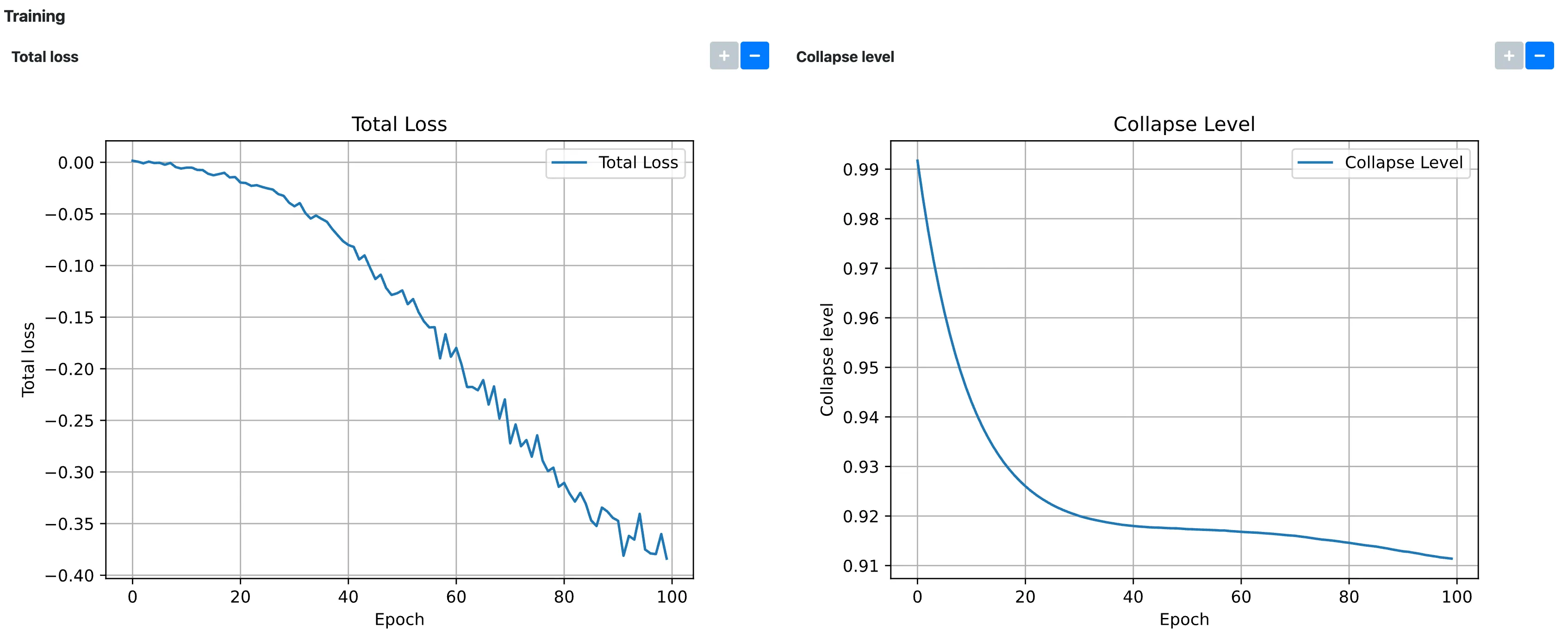
To check that the model has converged, we can check that the Total loss and Collapse level plots under the Training section have plateaued, ideally close to -1 and 0, respectively:

Selecting high-quality images by class ID (in nextPYP)¶

Using the clusters formed by K-Means, we can filter for high-quality clusters in the real and Fourier domains.
To exclude a cluster from further downstream processing, un-select the corresponding class number. You can do this for both the real and Fourier domains.
Once you are satisfied with your class ID selection, save your selection by naming a filter and clicking the Save icon.

Visualizing the learned embedding space (in Phoenix)¶

If, instead, you wish to interactively select your high-quality clusters using Phoenix, you can download the necessary files by clicking on the Download button in green for each domain.

Open a terminal on your local machine, activate your Phoenix conda environment, and decompress the *_prismpyp.tbz file:

cd $WORK_DIRECTORY
conda activate phoenix
tar xvfz *_prismpyp.tbz

You should now have 3 files: zipped_thumbnail_images.tar.gz, real/data_for_export.parquet, and fft/data_for_export.parquet.
Unzip the thumbnail images tarball:

mkdir -p thumbnail_images
tar -xvzf zipped_thumbnail_images.tar.gz -C thumbnail_images

Start a local HTTP server to host thumbnails:

cd $WORK_DIRECTORY
screen
python -m http.server 5004

In another terminal, download and launch the visualization script:

cd $WORK_DIRECTORY
conda activate phoenix
wget https://raw.githubusercontent.com/nextpyp/prismpyp/refs/heads/main/scripts/visualizer.py

python visualizer.py \
    real/data_for_export.parquet \
    --port 5004 \
    --which-embedding umap

Note

Make sure that the ports used in the preceeding two steps are identical!

When launched successfully, you should see output like:

🌍 To view the Phoenix app in your browser, visit http://localhost:54116/
📺 To view the Phoenix app in a notebook, run `px.active_session().view()`
📖 For more information on how to use Phoenix, check out https://docs.arize.com/phoenix

You can now access the interactive visualization at http://localhost:54116/.

Selecting high-quality images interactively (in Phoenix)¶

With Phoenix now running, click on the image_embeddings link to load the interactive visualization. Clicking on a point in the cloud will show the associated image in the bottom panel. You can also select a cluster of points using the left side bar (the corresponding image gallery will be shown at the bottom of the page).

Select the points or clusters of interest using the Select tool
Export your selection using the Export button and Download the results as a .parquet file

Note

You will need to make selections for both domains!

Go back to nextPYP, navigate to the Pre-processing block, and click on the prismPYP tab.
To upload the exported high-quality images from the real domain, click on the Upload button under the Real space tab, browse to the location of the .parquet file you exported from Phoenix, and upload the file.
Repeat the same process for the Fourier domain.
Unlike filtering by class ID, you do not have to save a filter in order to perform the intersection.

For more information about how to use Phoenix to make a selection, see the documentation here

Performing consensus filtering¶

Now that we have identified high-quality features in both domains, we can take the intersection of both sets of images to filter out bad micrographs.

Click on Particles (output of the Pre-processing block) and select Particle refinement
If you selected good class IDs in the Pre-processing block, select the filter you created by using the Filter micrographs (prismPYP) dropdown menu:

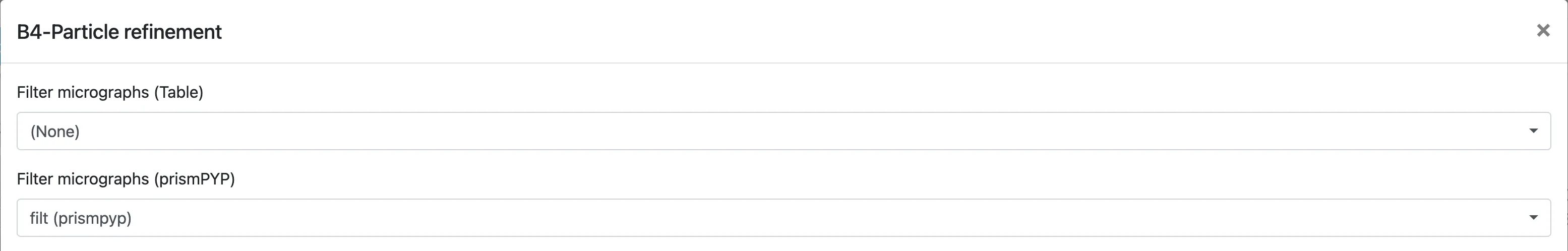
Otherwise, if you uploaded two .parquet files from Phoenix, you do not need to select any filters.
prismPYP filtering can be used in conjunction with traditional “table filtering” approaches. For more information on table filtering, see the documentation here.
In either case, when Particle refinement is executed, the first step will be to filter images before further processing.